Top Data Preprocessing Techniques for Machine Learning: Complete Guide with Examples
Introduction
If your machine learning model is not performing well, the problem is often not the algorithm — it’s the data.
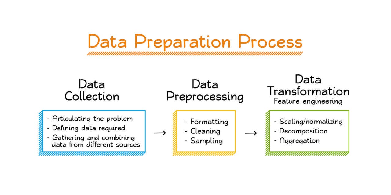
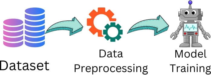
In real-world machine learning projects, raw data is usually messy, incomplete, inconsistent, and unstructured. That’s why data preprocessing is one of the most important steps in building an effective ML model.
In fact, many data scientists say:
70–80% of the work in machine learning is data cleaning and preprocessing.
In this guide, you will learn the most important data preprocessing techniques used in machine learning, explained in simple language with practical examples.
Quick Overview of Data Preprocessing Steps
| Step | Purpose | Example |
|---|---|---|
| Data Cleaning | Remove errors and inconsistencies | Remove duplicates |
| Feature Scaling | Normalize numerical values | MinMaxScaler |
| Encoding | Convert categorical text into numbers | One-Hot Encoding |
| Splitting | Divide data into training and testing sets | 80/20 split |
1. Data Cleaning
Data cleaning refers to the process of detecting and correcting (or removing) corrupt, inaccurate, or unnecessary data from a dataset. It is the foundation of data preprocessing because data from real-world sources is often messy, incomplete, or incorrect.
Key Aspects of Data Cleaning:
Handling Missing Data: Datasets may have missing entries, which can negatively affect model training. Missing data must be dealt with carefully to avoid bias in predictions. Common strategies include:
- Removing Data: Dropping rows or columns with missing values (if the percentage of missing data is small).
- Imputation: Filling in missing values with the mean, median, mode, or using more complex models (e.g., K-Nearest Neighbors or regression) to predict missing values.
Example of Imputation:
Here is a simple Python example:pythonfrom sklearn.impute import SimpleImputer import numpy as np # Sample dataset with missing values data = np.array([[1, 2], [np.nan, 3], [7, 6]]) # Impute missing values using the mean imputer = SimpleImputer(strategy='mean') imputed_data = imputer.fit_transform(data) print(imputed_data)Removing Duplicates: Duplicate records can distort analysis and model training. Identifying and removing them ensures data integrity.
Outlier Detection: Outliers are data points that differ significantly from the rest of the dataset and may skew the model’s results. Techniques like z-score, IQR (Interquartile Range), or visualizations like box plots are used to identify and remove outliers.
2. Handling Missing Data
Missing data can cause significant issues, particularly in machine learning models. Deciding how to handle missing data depends on the nature of the dataset and the amount of missing information.
Common Techniques to Handle Missing Data:
Listwise Deletion (Removing Data): This involves removing rows or columns with missing values. It is suitable when a small portion of the data is missing.
Imputation: Predicting or estimating missing values with statistical methods such as:
- Mean, Median, or Mode Imputation: Filling missing values with the average or most frequent value of the column.
- KNN Imputation: Using the values from the nearest neighbors to predict the missing data.
Interpolation: Estimating missing values by assuming the missing data lies between the known data points.
3. Feature Scaling
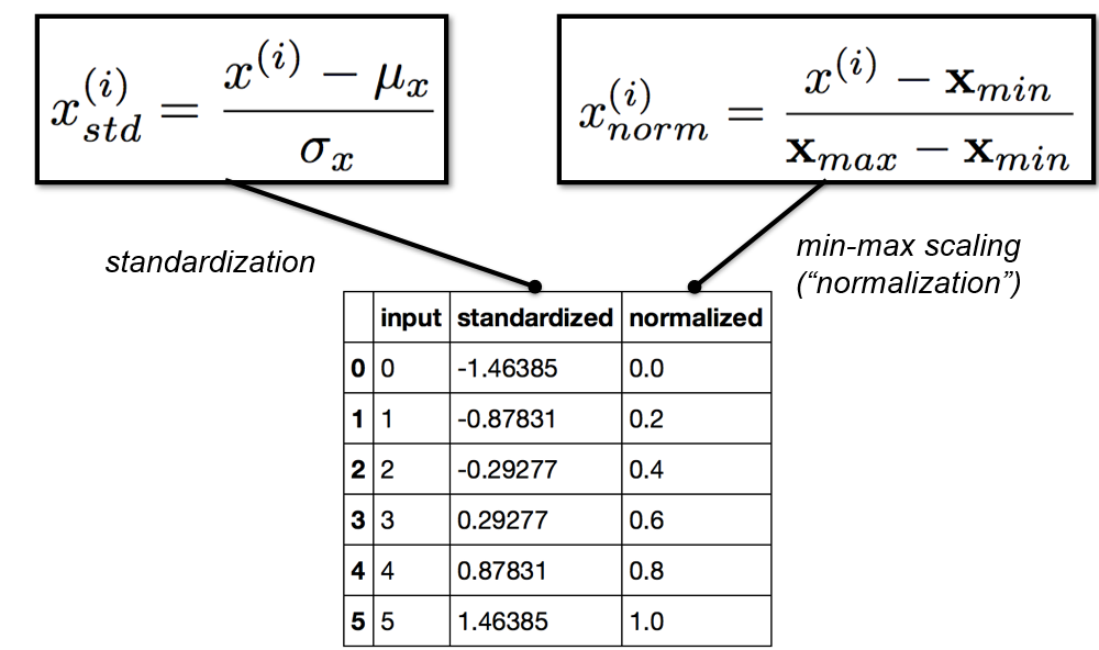
Feature scaling ensures that all the numerical values in a dataset are on the same scale, which is crucial for algorithms that calculate distances between data points, such as k-Nearest Neighbors, or for algorithms like gradient descent to converge faster.
Two Common Feature Scaling Techniques:
Normalization: Also known as Min-Max Scaling, it scales the data to a fixed range, usually between 0 and 1. This is useful when the algorithm doesn’t assume any distribution of the data (e.g., neural networks).
Example of Normalization
Here is a simple Python example:from sklearn.preprocessing import MinMaxScaler data = [[100, 0.2], [200, 0.4], [300, 0.6]] scaler = MinMaxScaler() scaled_data = scaler.fit_transform(data) print(scaled_data)Standardization: This technique transforms data so that it has a mean of 0 and a standard deviation of 1. It is most suitable when the data follows a normal (Gaussian) distribution and is widely used in algorithms like SVM, logistic regression, and linear regression.
- Formula: X_scaled = (X - Mean) / Standard Deviation
4. Feature Encoding
Many machine learning algorithms require numerical inputs, so categorical (non-numeric) data must be encoded into numerical form. This process is known as feature encoding.
Common Encoding Techniques:
- Label Encoding: Converts each unique category into a numerical value. This is a simple method but can lead to problems if the algorithm interprets these numbers as having an ordinal relationship.
- Example:
- One-Hot Encoding: Transforms each category into a separate binary column (0 or 1). This avoids the issue of false ordinality but can increase the number of columns, especially for datasets with many categories.
- Example:
Here is a simple Python example:from sklearn.preprocessing import OneHotEncoder
import numpy as np

data = [['Red'], ['Blue'], ['Green']]
encoder = OneHotEncoder()
encoded_data = encoder.fit_transform(data).toarray()
print(encoded_data)
5. Feature Selection
Feature selection involves identifying the most relevant features for your model and discarding irrelevant or redundant ones. Reducing the number of features helps simplify the model, improve performance, and avoid overfitting.
Types of Feature Selection Methods:
Filter Methods: These methods use statistical techniques to evaluate the relevance of each feature independently of the model. Correlation, Chi-square, and variance threshold are common techniques.
Wrapper Methods: These methods evaluate multiple combinations of features by running the model on each subset and selecting the best one. Recursive Feature Elimination (RFE) is a popular example.
Embedded Methods: Feature selection is done during the model training process itself. Lasso (L1 regularization) is an example, as it reduces the number of features by penalizing the model's complexity.
6. Data Splitting
Splitting the dataset into separate parts is critical for training and evaluating machine learning models. Typically, data is divided into three sets:
Training Set: Used to train the model. It usually consists of 70-80% of the data.
Validation Set: Used to fine-tune model hyperparameters and validate the model’s performance during training.
Test Set: A separate, unseen dataset used to evaluate the final performance of the model.
7. Dimensionality Reduction
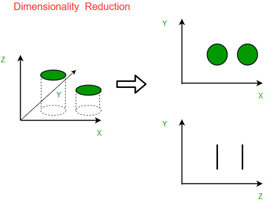
As datasets grow in size and complexity, they often contain many features. High-dimensional data can lead to overfitting and increased computational time. Dimensionality reduction techniques reduce the number of features while retaining the essential information.
Popular Techniques:
Principal Component Analysis (PCA): PCA is a statistical technique that transforms the original features into a smaller set of new variables (called principal components) while preserving as much variability as possible.
Linear Discriminant Analysis (LDA): LDA is a supervised technique used to find the linear combinations of features that best separate different classes.
8. Data Transformation
Data transformation refers to applying mathematical or statistical modifications to the dataset to improve the model’s performance.
Common Transformations:
Log Transformation: Applied to skewed data to reduce variability or the impact of outliers.
Polynomial Features: Generates new features based on polynomial combinations of the original features. This is useful for non-linear models.
9. Data Augmentation
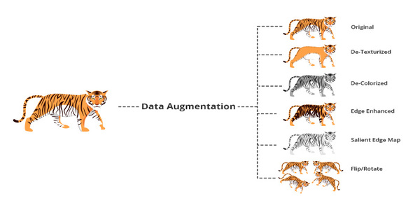
Data augmentation is a technique primarily used in domains like image and text data to artificially increase the size of the dataset by modifying existing data. For example, in image data, augmentations include rotating, flipping, or adding noise to the images. This helps prevent overfitting by making the model more robust to different variations of the data.
When Should You Focus on Preprocessing?
-
When your model accuracy is unexpectedly low
-
When your dataset contains missing or inconsistent values
-
When numerical features are on very different scales
-
When your dataset contains categorical variables
When your model accuracy is unexpectedly low
When your dataset contains missing or inconsistent values
When numerical features are on very different scales
When your dataset contains categorical variables
Conclusion
Data preprocessing is one of the most crucial steps in building effective machine learning models. Properly cleaning, scaling, and encoding the data, as well as selecting the right features, ensures the model performs well and makes accurate predictions. By mastering these preprocessing techniques, you can significantly improve your model’s performance and reliability, setting a strong foundation for machine learning success.



Often, data preprocessing is the unsung hero when it comes to machine learning! This article describes the basic techniques that are make or break when determining the accuracy of your models. I know from experience working with different datasets how crucial good preprocessing is. In fact, I have seen top app development company in usa use these techniques in their ML powered mobile apps – all seamlessly and accurate predictions. I am very glad the author emphasized the importance of data preprocessing in machine learning.
ReplyDeleteThank you! I completely agree—data preprocessing is the foundation of any successful machine learning model. It’s great to hear that you’ve seen its impact firsthand in real-world applications, especially in ML-powered mobile apps. Proper preprocessing ensures cleaner data, better feature representation, and ultimately, more accurate predictions. I appreciate your insights! 🚀
Delete